Plot and compare impulse responses from two estimation approaches

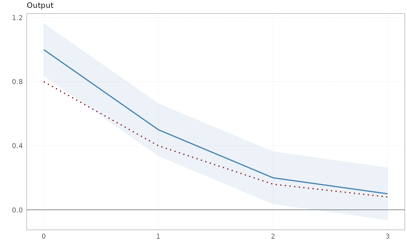
Produces a panel of IRF plots comparing two sets of impulse responses with normal confidence bands at level ci. This function is kept for backward compatibility and is a thin wrapper around plotirf(), which accepts up to three sets of impulse responses as well as bootstrap draws.

Usage

plot2irf(IRF1, IRF1se, IRF2, IRF2se, HTick, Labels, ci = 0.9)

Arguments

IRF1

Array (H x N x E) of impulse responses for the first approach. Dimnames on the first dimension must be the horizon labels (numeric).

IRF1se

Array (H x N x E) of standard errors for the first approach (set to 0 to suppress confidence intervals).

IRF2

Array (H x N x E) of impulse responses for the second approach.

IRF2se

Array (H x N x E) of standard errors for the second approach (set to 0 to suppress confidence intervals).

HTick

Integer. Step size for x-axis tick marks.

Labels

Character vector of length N. Variable names used as panel titles.

ci

Numeric scalar in (0, 1). Confidence level for the shaded bands. Defaults to 0.90 (90% CI).

Value

A list of ggplot objects, one per variable-shock combination, ordered by shock (outer loop) then variable (inner loop).

See also

plotirf()

Examples

irf1 <- array(c(1, 0.5, 0.2, 0.1), dim = c(4, 1, 1))
dimnames(irf1)[[1]] <- 0:3
irf2 <- irf1 * 0.8
se <- array(0.1, dim = dim(irf1), dimnames = dimnames(irf1))
plot2irf(irf1, se, irf2, se * 0, HTick = 1, Labels = "Output")
#> [[1]]

#>