Estimating Dynamic Causal Effects with hetiv

Introduction

hetiv provides tools for measuring and identifying multi-dimensional structural shocks in dynamic models models using two complementary IV approaches:

Heteroskedasticity-IV (Rigobon 2003, Rigobon and Sack 2004, Lewis 2022, Burri and Kaufmann, 2026a): exploits the higher variance of outcome variables on policy event days relative to control days to identify structural shocks without requiring external instruments.
Proxy-IV (Mertens and Ravn 2013, Stock and Watson 2018): uses an external instrument (proxy) that is correlated with the shock of interest but uncorrelated with other shocks.

Both approaches are implemented as local projection IV estimators following Jordà (2005), which directly produce impulse response functions (IRFs) across multiple horizons. Inference is based on HC robust standard errors (Montiel Olea et al., 2025).

The package allows for multiple shocks and endogenous variables. Weak-instrument HAR inference is implemented via the generalised minimum eigenvalue test of Lewis and Mertens (2025), which nests the classical Stock-Yogo (2005) test for the univariate homoskedastic case. gweakivtestis a direct port of the Matlab files by Lewis and Mertens (2025) available on https://karelmertens.com/research/.

In addition, the package provides the function kfpredict() for predicting the underlying unobserved shocks based on the Kalman-filter, as suggested by Burri and Kaufmann (2026b).

This vignette demonstrates the functionality using a simulated four-variable VAR with two structural shocks.

Simulated data

We simulate data from a VAR(2) with $N = 4$ variables, $E = 2$ event (policy) shocks, $R = 2$ regular shocks, and $P = 2$ lags over $T = 500$ observations. The model reads:

$y_t = \Psi \varepsilon_t + \Gamma v_t + \Phi(L) y_{t-1} + \beta X_t \ \ \text{for } t\in \mathcal{P}$

$y_t = \Gamma v_t + \Phi(L) y_{t-1} + \beta X_t \ \ \text{for } t\in \mathcal{C}$

where $\mathcal{P}, \mathcal{C}$ denote policy event and other days, respectively, $\Psi$ is the impact matrix of $E$ policy event shocks and $\Gamma$ the impact matrix of $R$ other shocks. $\Phi(L)$ is a conformable lag polynomial, and $X_t$ an matrix of deterministic terms.

Regular shocks occur on all days. A policy event occurs every 10th period (approximately 10% of observations). The latter introduces heteroskedasticity in the variance-covariance matrix of the reduced-form residuals hetiv() exploits to identify the impulse response functions. Shocks are drawn from a standard normal distribution. The impact matrix is lower-triangular, corresponding to the identifying assumption by Burri and Kaufmann (2026a) that the first shock has a contemporaneous effect on all variables, while the second shock has no contemporaneous effect on the first variable. Deterministic weekday patterns are added to variables 3 and 4 to illustrate the role of controls. The event indicator Ind equals 1 on policy event days and 0 on control days.

library(hetiv)

# Dimensions
N  <- 4   # variables
E  <- 2   # event shocks
R  <- 2   # regular shocks
P  <- 2   # VAR lag order
H  <- 20  # IRF horizons
Nevn <- 10 # Frequency of event shocks

# Impact matrix for event shocks (N x E); lower triangular for recursive ID
PsiE      <- matrix(0, N, E)
PsiE[, 1] <- c(1.0,  0.5,  0.3,  0.2)
PsiE[, 2] <- c(0.0,  1.0,  -0.4,  0.3)

SigE <- 4  # event shock variance (scalar, applies to all E shocks)

# Impact matrix for regular shocks (N x R)
PsiR      <- matrix(0, N, R)
PsiR[, 1] <- c( 1.0, -0.3,  0.2,  0.1)
PsiR[, 2] <- c( 0.2,  1.0, -0.1,  0.4)

# VAR coefficient matrices at lags 1 and 2
Phi       <- array(0, dim = c(N, N, P))
Phi[,, 1] <- matrix(c( 0.60,  0.05, -0.04,  0.03,
                        0.06,  0.40,  0.05, -0.03,
                       -0.05,  0.04,  0.50,  0.06,
                        0.03, -0.03,  0.05,  0.70), N, N, byrow = TRUE)
Phi[,, 2] <- matrix(c( 0.10,  0.03, -0.02,  0.02,
                        0.04,  0.10,  0.03, -0.02,
                       -0.03,  0.02,  0.10,  0.03,
                        0.02, -0.02,  0.03,  0.10), N, N, byrow = TRUE)

# Simulate — seed is set internally by simulatedata()
Nobs <- 500
Nbin <- 100
sim  <- simulatedata(
  Phi = Phi, SigE = SigE, PsiE = PsiE, PsiR = PsiR,
  Nobs = Nobs, Nbin = Nbin, N = N, R = R, E = E,
  Nevn = Nevn, P = P, eDist = 0, seed = 42
)

# Extract simulated data and event indicator
y_data <- sim$y
Ind    <- as.integer(sim$IndE[, 1])

# Add deterministic weekday variation into variables 3 and 4
y_data[, 3] <- y_data[, 3] + 0.5 * seq_len(Nobs) %% 5
y_data[, 4] <- y_data[, 4] + 0.3 * seq_len(Nobs) %% 5

To illustrate the proxy-IV approach, we construct a noisy external instrument for the two event shocks by adding Gaussian noise to the true shocks. The proxy is observed only on policy event days and set to NA on control days. This mirrors the typical situation in high-frequency identification of monetary policy shocks, where the high-frequency surprises are only observed on policy announcement days.

# RNG state after simulatedata(seed = 42) is deterministic, so no extra seed needed
e_proxy       <- sim$eE
e_proxy[, 1]  <- e_proxy[, 1] + rnorm(Nobs, sd = 1)
e_proxy[, 2]  <- e_proxy[, 2] + rnorm(Nobs, sd = 1)
e_proxy[Ind == 0, ] <- NA

Estimation

Heteroskedasticity-IV without controls

First, we estimate a misspecified model, failing to control for lagged dependent variables and weekday-variation. Note that we impose a normalization on the impact on the endogenous variable for every shock. The value of the normalization can be chosen by norm. Here, we choose the normalization that corresponds to the true impact matrix.

res_het <- hetiv(
  y       = y_data,
  O       = y_data,
  Ind     = Ind,
  P       = 0,
  H       = H,
  E       = E,
  norm    = 1,
  details = TRUE
)

Heteroskedasticity-IV with controls

Second, we estimate the correctly specified model, with $P = 2$ lags and the weekday dummies. Note that the weekday dummies absorb the deterministic pattern that we added to the data. The regressions generally include a constant term. Therefore, we only add four weekday dummies.


# Weekday dummies: four indicator variables (one left out as reference)
X_data <- matrix(0, nrow = Nobs, ncol = 4)
for (i in 1:4) X_data[, i] <- as.integer((seq_len(Nobs)) %% 5 == (i - 1))

res_het_X <- hetiv(
  y       = y_data,
  O       = y_data,
  X       = X_data,
  Ind     = Ind,
  P       = P,
  H       = H,
  E       = E,
  norm    = 1,
  details = TRUE
)

Proxy-IV

Third, we use the external instrument to estimate the model via proxy-IV. The same lags are included as in the second model. However, the weekday dummies are dropped due to collinearity, as only the event days are used to identify the responses. Note that the proxy-IV function still requires Ind as an input, because, in case the instrument is missing, but Ind = 1, we can later on predict the unobserved shock using the Kalman filter with kfpredict() (see Burri and Kaufmann, 2026a).

res_proxy <- proxyiv(
  y         = y_data,
  O         = y_data,
  Z         = e_proxy,
  Ind       = Ind,
  P         = P,
  H         = H,
  E         = E,
  norm      = 1,
  recursive = FALSE,
  details   = TRUE
)

Proxy-IV with recursive zero restriction

If the proxies are valid, we do not need additional restrictions to identify the impulse responses. However, the function allows us to additionally impose zero restrictions mirroring the assumptions used by hetiv(). This is useful in a situation where there is some doubt about the validity of the external instruments, and the researcher is convinced that a zero restriction is valid.

res_proxy_rec <- proxyiv(
  y         = y_data,
  O         = y_data,
  Z         = e_proxy,
  Ind       = Ind,
  P         = P,
  H         = H,
  E         = E,
  norm      = 1,
  recursive = TRUE,
  details   = TRUE
)

Impact matrices

The estimated impact matrix $\Psi$ gives the contemporaneous responses of all $N$ variables to each structural shock. We can compare the estimates across the four specifications against the true $\Psi$ . At first sight, the differences are small. As we will see below, there are still some differences in terms of the accuracy of the estimates, the predicted shocks, and the strength of the instruments.


tab_1 <- round(data.frame(
            True = PsiE[, 1], 
            HET_IV = res_het$Psi[, 1], 
            HET_IV_X = res_het_X$Psi[, 1],
            Proxy_IV = res_proxy$Psi[, 1], 
            Proxy_IV_rec = res_proxy_rec$Psi[, 1]), 2)

knitr::kable(
  tab_1,
  col.names = c("True", "HET-IV without controls", "HET-IV with controls", "Proxy-IV with controls", "Proxy-IV with recursive restriction"),
  caption   = "Impact matrix estimates ($\\Psi$) for shock 1 across different specifications"
)

Impact matrix estimates ( $\Psi$ ) for shock 1 across different specifications
True	HET-IV without controls	HET-IV with controls	Proxy-IV with controls	Proxy-IV with recursive restriction
1.0	1.00	1.00	1.00	1.00
0.5	0.53	0.45	0.53	0.53
0.3	0.52	0.31	0.29	0.29
0.2	0.20	0.19	0.22	0.22


tab_2 <- round(data.frame(
            True = PsiE[, 2], 
            HET_IV = res_het$Psi[, 2], 
            HET_IV_X = res_het_X$Psi[, 2],
            Proxy_IV = res_proxy$Psi[, 2], 
            Proxy_IV_rec = res_proxy_rec$Psi[, 2]), 2)

knitr::kable(
  tab_2,
  col.names = c("True", "HET-IV without controls", "HET-IV with controls", "Proxy-IV with controls", "Proxy-IV with recursive restriction"),
  caption   = "Impact matrix estimates ($\\Psi$) for shock 2 across different specifications"
)

Impact matrix estimates ( $\Psi$ ) for shock 2 across different specifications
True	HET-IV without controls	HET-IV with controls	Proxy-IV with controls	Proxy-IV with recursive restriction
0.0	0.00	0.00	-0.09	0.00
1.0	1.00	1.00	1.00	1.00
-0.4	-0.46	-0.31	-0.35	-0.31
0.3	0.26	0.31	0.28	0.28

Impulse response functions

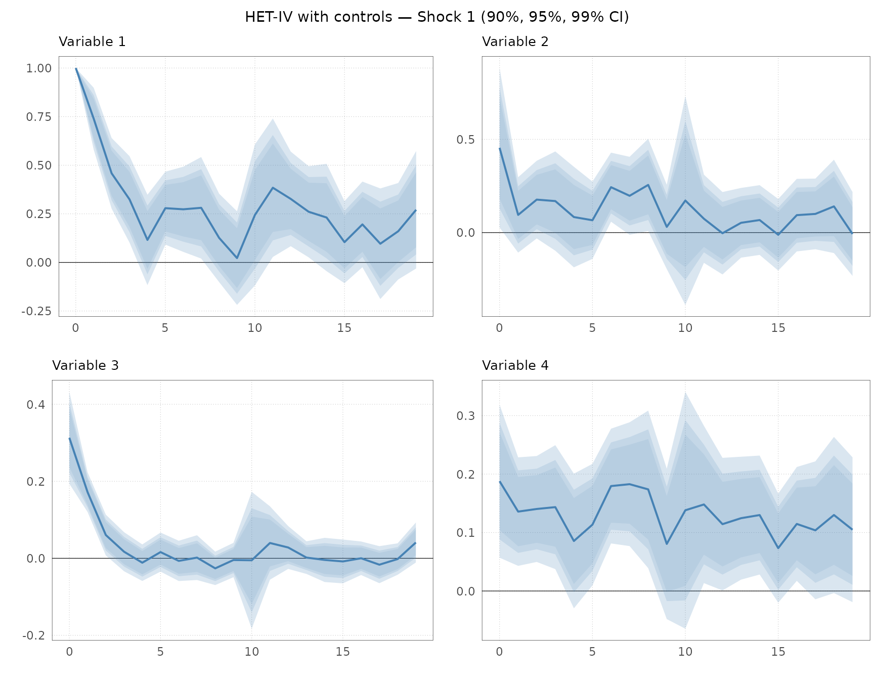
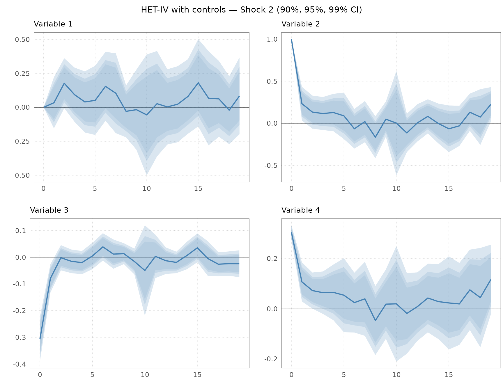
Impulse responses with confidence intervals

We can assess the accuracy of the estimates, and the dynamic causal effects, using plotirf(). The function plots IRFs with shaded confidence bands for one estimation approach. The confidence levels can be chosen freely. Here, we show the 90%, 95%, and 99% confidence intervals for the HET-IV estimates with controls.

var_labels <- paste0("Variable ", 1:N)

plots_het_X <- plotirf(
  IRFest = res_het_X$irf,
  IRFse  = res_het_X$se,
  HTick  = 5,
  Labels = var_labels,
  ci     = c(0.90, 0.95, 0.99)
)

for (j in seq_len(E)) {
  idx   <- ((j - 1) * N + 1):(j * N)
  panel <- cowplot::plot_grid(plotlist = plots_het_X[idx], ncol = 2)
  title <- cowplot::ggdraw() +
    cowplot::draw_label(paste0("HET-IV with controls — Shock ", j, " (90%, 95%, 99% CI)"), size = 11)
  print(cowplot::plot_grid(title, panel, ncol = 1, rel_heights = c(0.05, 1)))
}

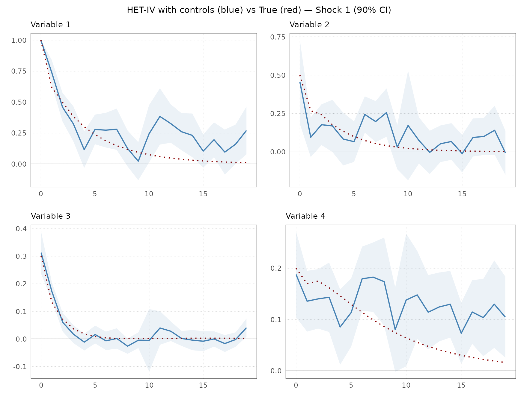
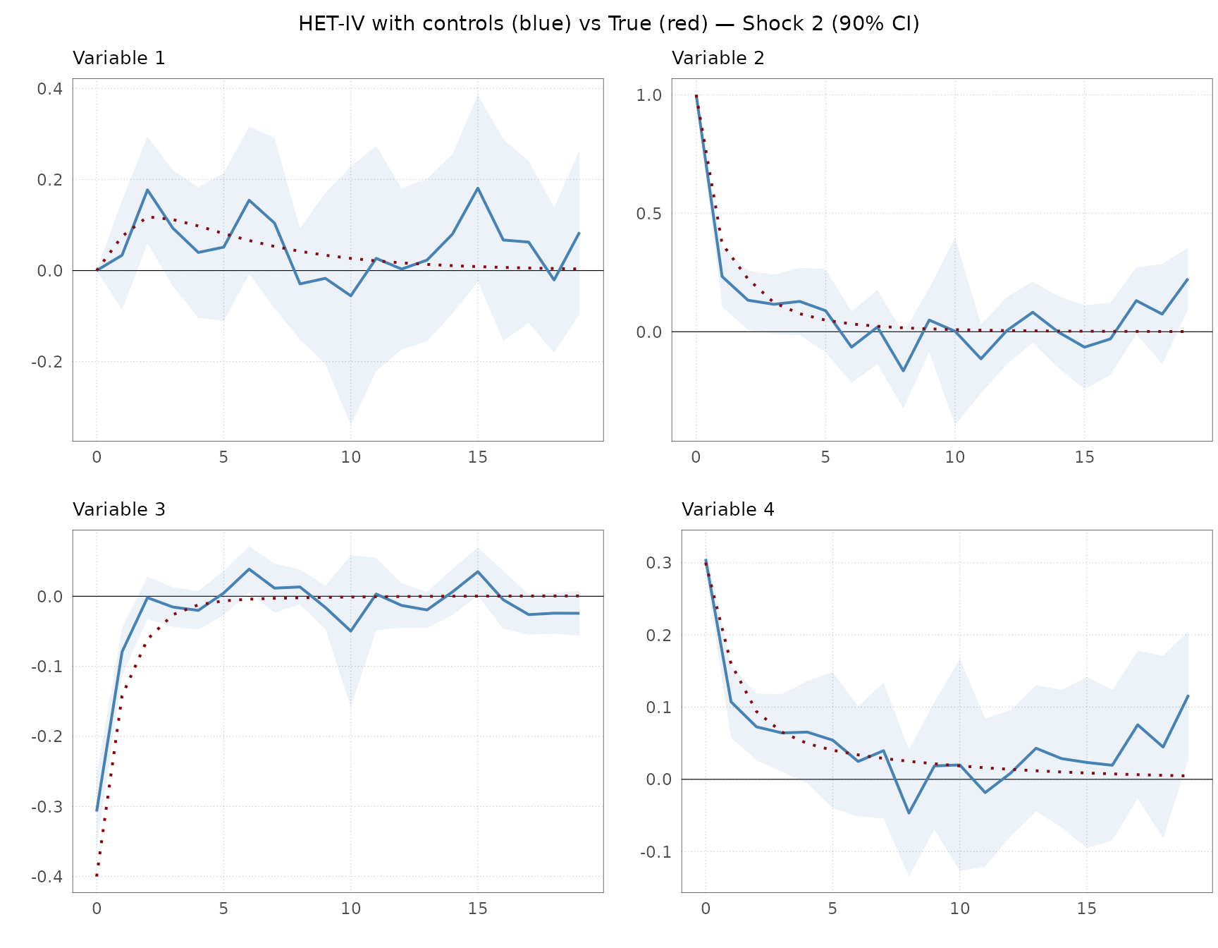
HET-IV estimates versus true IRF

We can compare the estimates to the true impulse responses. plot2irf() overlays two sets of IRFs. We compare the HET-IV estimate (blue) against the theoretical IRF computed from the known VAR parameters (red). The function computeirf() computes the theoretical IRF. The standard errors for the true IRF are set to zero, so that no confidence bands are plotted for the true IRF.

irf_true    <- computeirf(PsiE, Phi, H, cum = FALSE)
irf_true_se <- array(0, dim = dim(irf_true), dimnames = dimnames(irf_true))

plots_vs_true <- plot2irf(
  IRF1   = res_het_X$irf,
  IRF1se = res_het_X$se,
  IRF2   = irf_true,
  IRF2se = irf_true_se,
  HTick  = 5,
  Labels = var_labels,
  ci     = 0.90
)

for (j in seq_len(E)) {
  idx   <- ((j - 1) * N + 1):(j * N)
  panel <- cowplot::plot_grid(plotlist = plots_vs_true[idx], ncol = 2)
  title <- cowplot::ggdraw() +
    cowplot::draw_label(
      paste0("HET-IV with controls (blue) vs True (red) — Shock ", j, " (90% CI)"), size = 11)
  print(cowplot::plot_grid(title, panel, ncol = 1, rel_heights = c(0.05, 1)))
}

HET-IV estimates versus misspecified model

We can also compare the accuracy of the estimates using the correct and misspecified models.


plots_vs_true <- plot2irf(
  IRF1   = res_het_X$irf,
  IRF1se = res_het_X$se,
  IRF2   = res_het$irf,
  IRF2se = res_het$se,
  HTick  = 5,
  Labels = var_labels,
  ci     = 0.90
)

for (j in seq_len(E)) {
  idx   <- ((j - 1) * N + 1):(j * N)
  panel <- cowplot::plot_grid(plotlist = plots_vs_true[idx], ncol = 2)
  title <- cowplot::ggdraw() +
    cowplot::draw_label(
      paste0("HET-IV with controls (blue) vs without controls (red) — Shock ", j, " (90% CI)"), size = 11)
  print(cowplot::plot_grid(title, panel, ncol = 1, rel_heights = c(0.05, 1)))
}

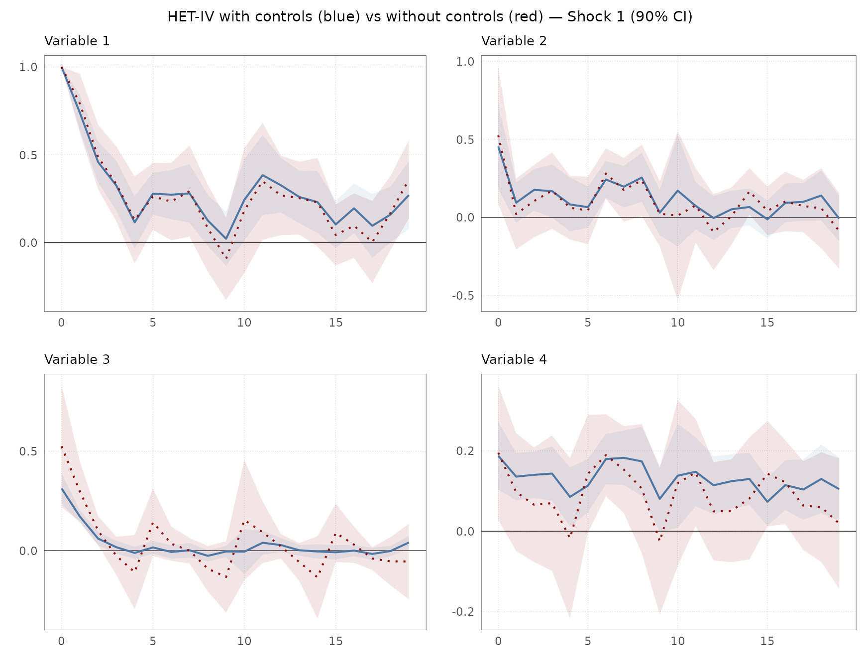
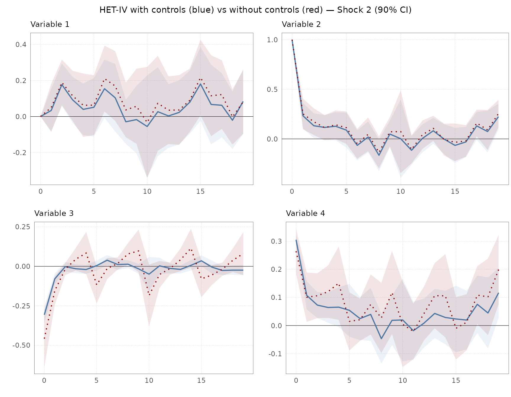
We see that the confidence intervals are wider using the misspecified model (red). This is especially true for the third and fourth variables that are affected by the deterministic weekday pattern. The misspecified model does not account for this pattern, which leads to more uncertainty and biased estimates. But also, the intervals are somewhat wider or variables 1 and 2 because we fail to control for lagged dependent variables.

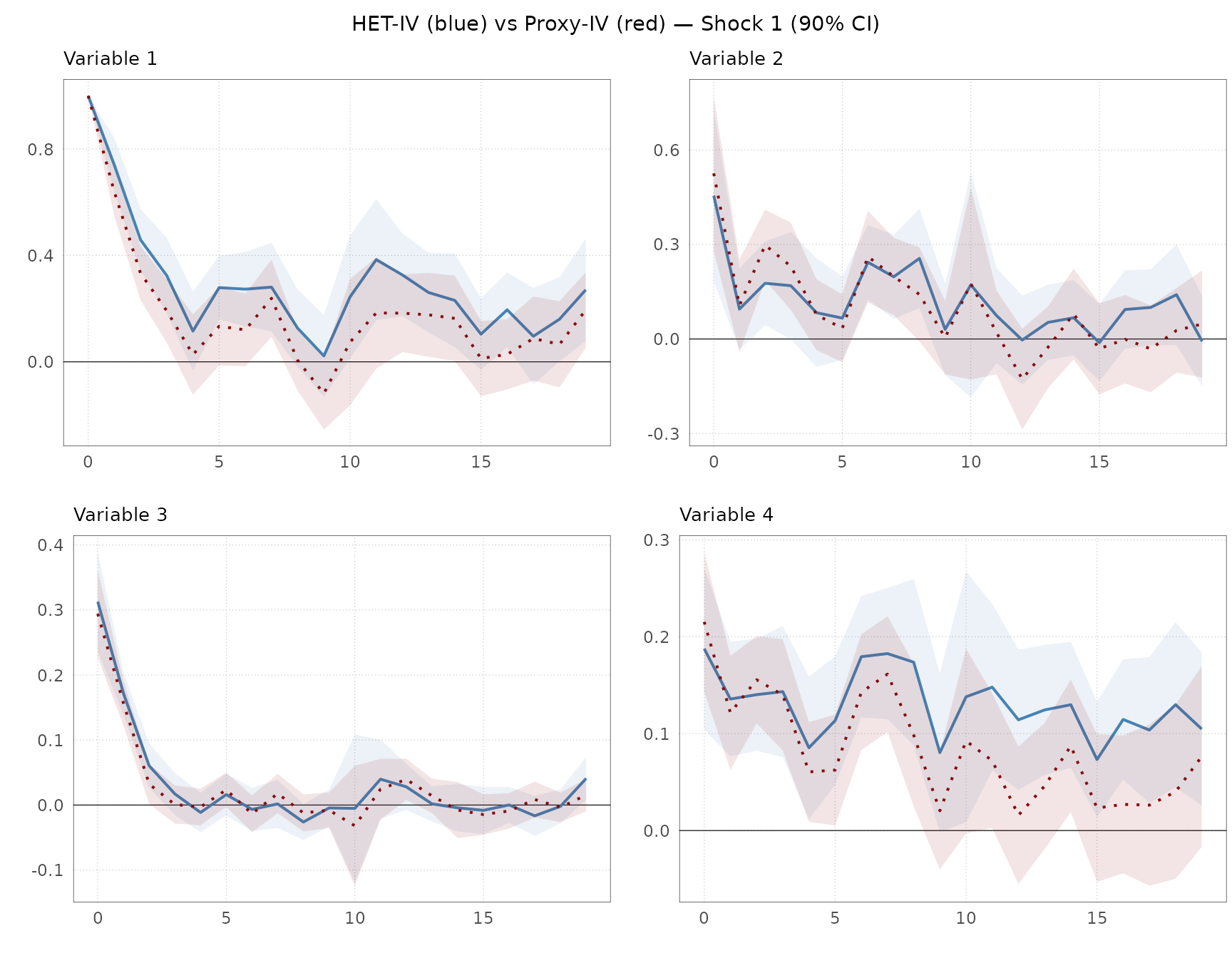
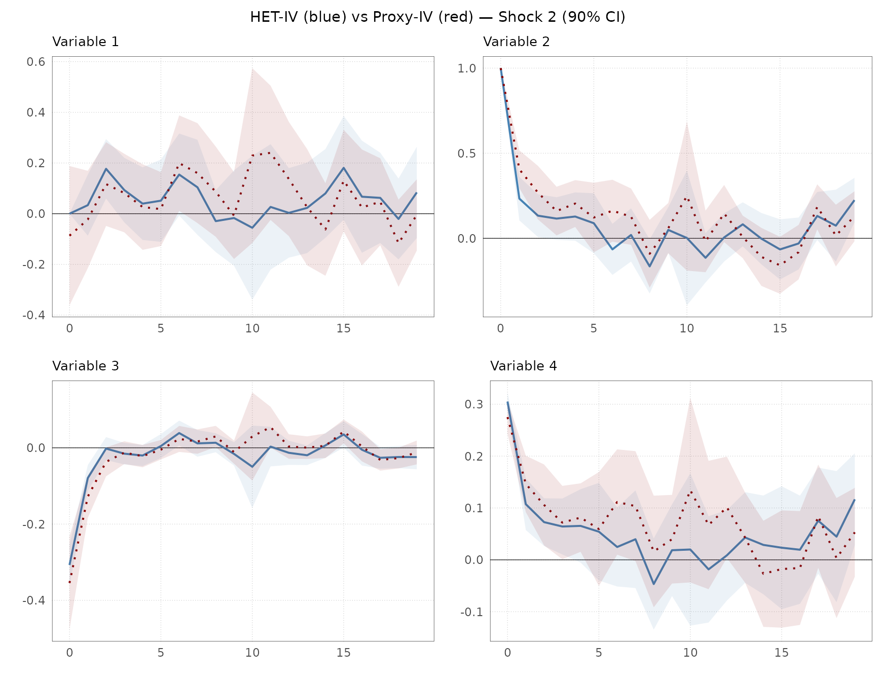
HET-IV versus Proxy-IV

Next, we compare the HET-IV estimates to the Proxy-IV estimates. We obtain relatively similar results with both approaches.However, the point estimates are quite similar across the two approaches.

plots_vs_proxy <- plot2irf(
  IRF1   = res_het_X$irf,
  IRF1se = res_het_X$se,
  IRF2   = res_proxy$irf,
  IRF2se = res_proxy$se,
  HTick  = 5,
  Labels = var_labels,
  ci     = 0.90
)

for (j in seq_len(E)) {
  idx   <- ((j - 1) * N + 1):(j * N)
  panel <- cowplot::plot_grid(plotlist = plots_vs_proxy[idx], ncol = 2)
  title <- cowplot::ggdraw() +
    cowplot::draw_label(
      paste0("HET-IV (blue) vs Proxy-IV (red) — Shock ", j, " (90% CI)"), size = 11)
  print(cowplot::plot_grid(title, panel, ncol = 1, rel_heights = c(0.05, 1)))
}

Shock extraction

kfpredict() recovers structural shocks from reduced-form residuals via a Kalman filter prediction. It requires the estimated impact matrix Psi, the residual covariance matrices on event and control days (Sig, SigR), and the residuals et.

shocks_het   <- kfpredict(Sig = res_het$Sig,   SigR = res_het$SigR,
                           Psi = res_het$Psi,   et   = res_het$et)

shocks_het_X <- kfpredict(Sig = res_het_X$Sig, SigR = res_het_X$SigR,
                           Psi = res_het_X$Psi, et   = res_het_X$et)

shocks_proxy <- kfpredict(Sig = res_proxy$Sig, SigR = res_proxy$SigR,
                           Psi = res_proxy$Psi, et   = res_proxy$et)

shocks_proxy_rec <- kfpredict(Sig = res_proxy_rec$Sig, SigR = res_proxy_rec$SigR,
                           Psi = res_proxy_rec$Psi, et   = res_proxy_rec$et)

We assess the accuracy of the prediction comparing them to the true event shocks from the underlying model.

true_shocks <- sim$eE

cor_df1<- data.frame(
    True       = true_shocks[, 1],
    Proxy      = e_proxy[, 1],
    HET_IV     = shocks_het[, 1],
    HET_IV_X   = shocks_het_X[, 1],
    Proxy_IV_X = shocks_proxy[, 1],
    Proxy_IV_Rec = shocks_proxy_rec[, 1]
)

cor_df2<- data.frame(
    True       = true_shocks[, 2],
    Proxy      = e_proxy[, 2],
    HET_IV     = shocks_het[, 2],
    HET_IV_X   = shocks_het_X[, 2],
    Proxy_IV_X = shocks_proxy[, 2],
    Proxy_IV_Rec = shocks_proxy_rec[, 2]
)

tab_all <- data.frame(
      rbind(round(cor(cor_df1, use = "complete.obs"), 2)[1, ],
            round(cor(cor_df2, use = "complete.obs"), 2)[1, ])
            )
rownames(tab_all) <- c("Shock 1", "Shock 2")

knitr::kable(tab_all,
    col.names = c("True", "Proxy", "HET-IV without controls", "HET-IV with controls", "Proxy-IV with controls", "Proxy-IV with recursive restriction"),
    row.names = TRUE,
    caption   = "Correlation of predicted shocks with true shocks"
    )

Correlation of predicted shocks with true shocks
	True	Proxy	HET-IV without controls	HET-IV with controls	Proxy-IV with controls	Proxy-IV with recursive restriction
Shock 1	1	0.91	0.70	1.00	0.98	0.98
Shock 2	1	0.80	0.85	0.94	0.89	0.88

The correlation between the true shocks and the proxy is slightly lower than one due to an attenuation bias (see Burri and Kaufmann, 2026a), which depends on the variance of the noise term affecting the proxy. The correlation of the prediction is also relatively low if we use a misspecified model. However, if we use the correct model, the correlation is is close to unity for Shock 1 and 0.94 for Shock 2. Proxy-IV with controls yields a high correlation as well, at least for Shock 1. Note that the specific values depend on the exact nature of the simulated data

Weak instrument test

gweakivtest() implements the generalised minimum eigenvalue test of Lewis and Mertens (2025), which is robust to heteroskedasticity and autocorrelation and applicable to multiple endogenous regressors and multiple instruments. Note that classical Stock-Yogo (2005) test is applicable only for the homoskedastic case.

Both hetiv() and proxyiv() return a WeakData object when details = TRUE. This data frame contains the data expected by gweakivtest(). The code below extracts the relevant columns from the WeakData data frame and runs the weak instrument test for each of the four specifications. For illustration, we use the heteroskedasticity-robust version (EHW). For the HAR (Newey West) version, use the option NW. By default, the function uses a bias tolerance of 10% at a significance level of 5%.

# Helper: extract y, Y, X, Z from WeakData and run gweakivtest
run_weaktest <- function(weakdata, E) {
  # y: outcome variable E+1 (not used as endogenous regressor)
  y <- weakdata[, paste0("y", E + 1)]
  # Y: first E outcome variables (endogenous regressors)
  Y <- weakdata[, paste0("y", 1:E)]
  # Z: the E instruments
  Z <- weakdata[, paste0("Z", 1:E),]
  # X: lagged ("o*") and deterministic ("x*") control columns. In any case, add a constant term as well.
  # Note that gweakivtest() adds a constant term if missing
  ctrl  <- startsWith(colnames(weakdata), "o") | startsWith(colnames(weakdata), "x") | startsWith(colnames(weakdata), "i")
  X     <- if (any(ctrl)) cbind(weakdata[, ctrl], matrix(1, nrow(weakdata), 1)) else matrix(numeric(0), nrow(weakdata), 0)

  gweakivtest(y, Y, X, Z, cov_type = "EHW")
}

specs <- list(
  "HET-IV, no controls"                            = res_het$WeakData,
  "HET-IV, with controls"                          = res_het_X$WeakData,
  "Proxy-IV, with controls"                        = res_proxy$WeakData,
  "Proxy-IV, with controls + recursive restriction" = res_proxy_rec$WeakData
)

wt_results <- lapply(specs, run_weaktest, E = E)

tab <- do.call(rbind, lapply(names(wt_results), function(nm) {
  r <- wt_results[[nm]]
  data.frame(
    Specification = nm,
    Statistic     = round(r$gmin_generalized, 2),
    LM_CV         = round(r$gmin_generalized_critical_value, 2),
    Strong        = ifelse(r$gmin_generalized > r$gmin_generalized_critical_value,
                           "Yes", "No"),
    stringsAsFactors = FALSE
  )
}))

knitr::kable(
  tab,
  col.names = c("Specification", "Statistic", "LM critical value",
                "Strong instruments?"),
  caption   = "Weak instrument test results (Lewis-Mertens generalised minimum eigenvalue test)"
)

Weak instrument test results (Lewis-Mertens generalised minimum eigenvalue test)
Specification	Statistic	LM critical value	Strong instruments?
HET-IV, no controls	15.55	38.28	No
HET-IV, with controls	88.68	47.23	Yes
Proxy-IV, with controls	23.03	23.27	No
Proxy-IV, with controls + recursive restriction	23.03	23.27	No

The specification without controls is affected by a weak instrument problem. The correctly specified model passes the weak instrument tests. The Proxy-IV fail the test. However, note that this depends on the degree of noise used to construct the proxy and is not suggesting that hetiv()is generally superior to proxyiv(). Interestingly, at least for HET-IV, the critical values are much higher than the common rule of thumb for the Stock and Yogo (2005) test, but also, higher than in the HAR test for the univariate case by Montiel Olea and Pflueger (2013) and Lewis (2022), which is around 23.

References

Burri, M. and Kaufmann, D. (2026a). Measuring monetary policy shocks. IRENE Working Papers 24-03, IRENE Institute of Economic Research, University of Neuchâtel.

Burri, M. and Kaufmann, D. (2026b). Multiple monetary policy shocks from daily data: A heteroskedasticity IV approach. IRENE Working Papers 26-06, IRENE Institute of Economic Research, University of Neuchâtel.

Jordà, Ò. (2005). Estimation and inference of impulse responses by local projections. American Economic Review, 95(1), 161–182.

Lewis, D. J. (2022). Robust inference in models identified via heteroskedasticity. Review of Economics and Statistics, 104(3), 510–524.

Lewis, D. J. and Mertens, K. (2025). A robust test for weak instruments for 2SLS with multiple endogenous regressors. The Review of Economic Studies, DOI: 10.1093/restud/rdaf103.

Mertens, K. and Ravn, M. O. (2013). The dynamic effects of personal and corporate income tax changes in the United States. American Economic Review, 103(4), 1212–1247.

Montiel Olea, J. L. and Pflueger, C. E. (2013). A robust test for weak instruments. Journal of Business & Economic Statistics, 31(3), 358-369.

Montiel Olea, J. L., M. Plagborg-Møller, E. Qian, C. K. Wolf (2025). Local projections or VARs? A primer for macroeconomists. NBER Macroeconomics Annual 2025, vol. 40, pp. 1-64, National Bureau of Economic Research.

Rigobon, R. (2003). Identification through heteroskedasticity. Review of Economics and Statistics, 85(4), 777–792.

Stock, J. H. and Watson, M. W. (2018). Identification and estimation of dynamic causal effects in macroeconomics using external instruments. Economic Journal, 128(610), 917–948.

Stock, J. H. and Yogo, M. (2005). Testing for weak instruments in linear IV regression. In D. W. K. Andrews and J. H. Stock (Eds.), Identification and inference for econometric models, pp. 80–108. Cambridge University Press.

Daniel Kaufmann, Marc Burri, Valentin Grob

2026-05-28